Scientific Programming with NumPy

Overview

Teaching: 15 min
Exercises: 65 min

Questions

• What is NumPy and what can I use it for?

• What are the differences between NumPy arrays and Python lists?

• How do I extract subsets of data from a dataset?

• How can I use NumPy to tell me basic statistical properties about my data?

Objectives

• Explain the key similarities and differences between NumPy arrays and Python lists.

• Select subsets of data from a NumPy array using Python slicing.

• Efficiently perform elementwise operations on data.

• Obtain basic characteristics of tabular data using NumPy’s statistical functions.

• Apply operations to differently sized arrays.

Introduction to NumPy (and Matplotlib)

See topic video lecture, and PowerPoint slides used with per-slide notes.

Adding NumPy to our Virtual Environment

In order to use NumPy, since it’s a third party Python external library we first need to install it. Since we’ve starting a new set of work for analysing data with this package, we should create a new virtual environment. We need to:

1. Open a new terminal (to ensure a fresh environment) and ensure we are in the correct directory to create our new virtual environment
2. Create a new virtual environment in that directory
3. Activate the virtual environment
4. Install the NumPy Python package to that environment

We can do this as follows:

cd
cd se-day2/code
python3 -m venv venv
source venv/bin/activate
pip3 install numpy

This reflects a typical way of working with virtual environments: a new project comes along, we create a new virtual environment in a location close to where we’re working (typically in the same directory as our code), we activate that virtual environment and install the packages we’ll need for the work.

NumPy Arrays vs Python Lists

Start the Python’s interpreter from the terminal again using python3 at the prompt. NumPy’s array type represents a multidimensional matrix M_i,j,k…n

The NumPy array seems at first to be just like a list:

import numpy as np
my_array = np.array(range(5))
my_array

Note here we are importing the NumPy module as np, an established convention for using NumPy which means we can refer to NumPy using np. instead of the slightly more laborious numpy..

array([0, 1, 2, 3, 4])

Ok, so they look like a list.

my_array[2]

2

We can access them like a list.

We can also access NumPy arrays as a collection in for loops:

for element in my_array:
    print("Hello" * element)

Hello
HelloHello
HelloHelloHello
HelloHelloHelloHello

However, we can also see our first weakness of NumPy arrays versus Python lists:

my_array.append(4)

Traceback (most recent call last):
  File "<stdin>", line 1, in <module>
AttributeError: 'numpy.ndarray' object has no attribute 'append'

For NumPy arrays, you typically don’t change the data size once you’ve defined your array, whereas for Python lists, you can do this efficiently. Also, NumPy arrays only contain one datatype. However, you get back lots of goodies in return…

Elementwise Operations

One great advantage of NumPy arrays is that most operations can be applied element-wise automatically, and in a very Pythonic way!

my_array + 2

+ in this context is an elementwise operation performed on all the matrix elements, and gives us:

array([2, 3, 4, 5, 6])

Other elementwise operations

Try using -, *, / in the above statement instead. Do they do what you expect?

Solution

my_array - 2
my_array * 2
my_array / 2

Will yield the following respectively:

array([-2, -1,  0,  1,  2])
array([0, 2, 4, 6, 8])
array([0. , 0.5, 1. , 1.5, 2. ])

Note the final one with / - digits after the . are omitted if they don’t show anything interesting (i.e. they are zero).

These are known as ‘vectorised’ operations, and are very fast.

But for now, let’s take a brief look at a basic example that demonstrates the performance of NumPy over Python lists. First, using Python lists we can do the following, that creates a 2D list of size 10000x10000, sets all elements to zero, then adds 10 to all those elements:

nested_list = [[0 for _ in range(10000)] for _ in range(10000)]
nested_list = [[x+10 for x in column] for column in nested_list]

That took a while! In NumPy we replicate this by doing:

import numpy as np
array = np.zeros((10000, 10000))
array = array + 10

Here, we import the NumPy library, use a specialised function to set up a NumPy array of size 5000x5000 with elements set to zero, and then - in a very Pythonic way - add 10 to each element. It’s simpler, closer to our conceptual model of what we want to achieve, and due to NumPy’s optimisations for dealing with matrices, it’s much faster.

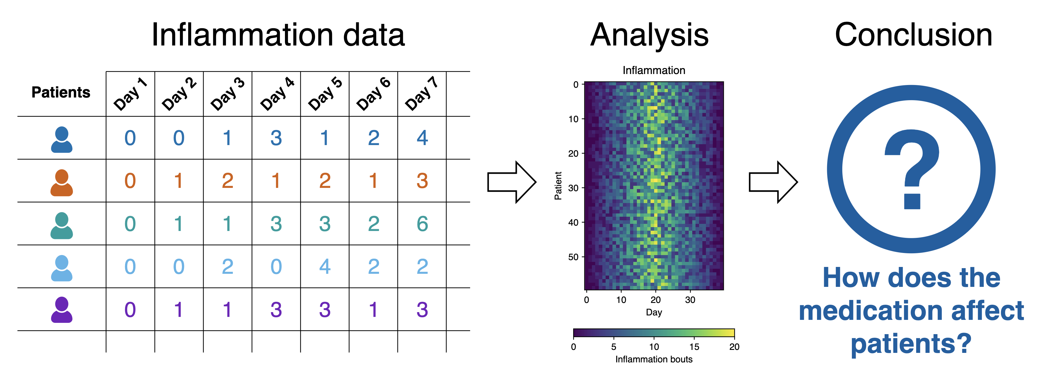
Introducing an Inflammation Dataset

We’re now going to use an example dataset based on a clinical trial of inflammation in patients who have been given a new treatment for arthritis. There are a number of these data sets in the data directory.

What Does the Patient Inflammation Data Contain?

Each dataset records inflammation measurements from a separate clinical trial of the drug, and each dataset contains information for 60 patients, who had their inflammation levels recorded for 40 days whilst participating in the trial.

Inflammation study pipeline from the Software Carpentry Python novice lesson

Each of the data files uses the popular comma-separated (CSV) format to represent the data, where:

• Each row holds inflammation measurements for a single patient,
• Each column represents a successive day in the trial,
• Each cell represents an inflammation reading on a given day for a patient (in some arbitrary units of inflammation measurement).

We can use first NumPy to load our dataset into a Python variable:

data = np.loadtxt(fname='../data/inflammation-01.csv', delimiter=',')
data

array([[0., 0., 1., ..., 3., 0., 0.],
       [0., 1., 2., ..., 1., 0., 1.],
       [0., 1., 1., ..., 2., 1., 1.],
       ...,
       [0., 1., 1., ..., 1., 1., 1.],
       [0., 0., 0., ..., 0., 2., 0.],
       [0., 0., 1., ..., 1., 1., 0.]])

So, the data in this case has 60 rows (one for each patient) and 40 columns (one for each day) as we would expect. Each cell in the data represents an inflammation reading on a given day for a patient. So this shows the results of measuring the inflammation of 60 patients over a 40 day period.

In the Corner

What may also surprise you is that when Python displays an array, it shows the element with index [0, 0] in the upper left corner rather than the lower left. This is consistent with the way mathematicians draw matrices but different from the Cartesian coordinates. The indices are (row, column) instead of (column, row) for the same reason, which can be confusing when plotting data.

Examining our Dataset

Let’s ask what type of thing data refers to:

print(type(data))

<class 'numpy.ndarray'>

The output tells us that data currently refers to an N-dimensional array, the functionality for which is provided by the NumPy library.

Data Type

A Numpy array contains one or more elements of the same type. The type function will only tell you that a variable is a NumPy array but won’t tell you the type of thing inside the array. We can find out the type of the data contained in the NumPy array.

print(data.dtype)

float64

This tells us that the NumPy array’s elements are 64-bit floating-point numbers.

With the following command, we can see the array’s shape:

print(data.shape)

(60, 40)

The output tells us that the data array variable contains 60 rows and 40 columns, as we would expect.

We can also access specific elements of our 2D array (such as the first value) like this:

data[0, 0]

0.0

Or the value in the middle of the dataset:

data[30, 20]

13.0

Slicing our Inflammation Data

An index like [30, 20] selects a single element of an array, but similar to how we slice lists, we can slice whole sections of NumPy arrays as well.

For example, we can select the first ten days (columns) of values for the first four patients (rows) like this:

data[0:4, 0:10]

array([[0., 0., 1., 3., 1., 2., 4., 7., 8., 3.],
       [0., 1., 2., 1., 2., 1., 3., 2., 2., 6.],
       [0., 1., 1., 3., 3., 2., 6., 2., 5., 9.],
       [0., 0., 2., 0., 4., 2., 2., 1., 6., 7.]])

So here 0:4 means, “Start at index 0 and go up to, but not including, index 4.” Again, the up-to-but-not-including takes a bit of getting used to, but the rule is that the difference between the upper and lower bounds is the number of values in the slice.

And as we saw with lists, we don’t have to start slices at 0:

data[5:10, 0:10]

Which will show us data from patients 5-9 (rows) across the first 10 days (columns):

array([[0., 0., 1., 2., 2., 4., 2., 1., 6., 4.],
       [0., 0., 2., 2., 4., 2., 2., 5., 5., 8.],
       [0., 0., 1., 2., 3., 1., 2., 3., 5., 3.],
       [0., 0., 0., 3., 1., 5., 6., 5., 5., 8.],
       [0., 1., 1., 2., 1., 3., 5., 3., 5., 8.]])

We also don’t have to include the upper and lower bound on the slice. If we don’t include the lower bound, Python uses 0 by default; if we don’t include the upper, the slice runs to the end of the axis, and if we don’t include either (i.e., if we just use ‘:’ on its own), the slice includes everything:

small = data[:3, 36:]
small

The above example selects rows 0 through 2 and columns 36 through to the end of the array:

array([[2., 3., 0., 0.],
       [1., 1., 0., 1.],
       [2., 2., 1., 1.]])

Numpy Memory

Numpy memory management can be tricksy:

x = np.arange(5)
y = x[:]

y[2] = 0
x

array([0, 1, 0, 3, 4])

It does not behave like lists!

x = list(range(5))
y = x[:]

y[2] = 0
x

[0, 1, 2, 3, 4]

We can use np.copy() to force the use of separate memory and actually copy the values. Otherwise NumPy tries its hardest to make slices be views on data, referencing existing values and not copying them. So an example using np.copy():

x = np.arange(5)
y = np.copy(x)
y[2] = 0
x

array([0, 1, 2, 3, 4])

Elementwise Operations on Multiple Arrays

As we’ve seen, arrays also know how to perform common mathematical operations on their values element-by-element:

doubledata = data * 2.0

Will create a new array doubledata, each element of which is twice the value of the corresponding element in data:

print('original:')
data[:3, 36:]
print('doubledata:')
doubledata[:3, 36:]

original:
array([[2., 3., 0., 0.],
       [1., 1., 0., 1.],
       [2., 2., 1., 1.]])
doubledata:
array([[4., 6., 0., 0.],
       [2., 2., 0., 2.],
       [4., 4., 2., 2.]])

If, instead of taking an array and doing arithmetic with a single value (as above), you did the arithmetic operation with another array of the same shape, the operation will be done on corresponding elements of the two arrays:

tripledata = doubledata + data

Will give you an array where tripledata[0,0] will equal doubledata[0,0] plus data[0,0], and so on for all other elements of the arrays.

print('tripledata:')
print(tripledata[:3, 36:])

tripledata:
array([[6., 9., 0., 0.],
       [3., 3., 0., 3.],
       [6., 6., 3., 3.]])

Stacking Arrays

Arrays can be concatenated and stacked on top of one another, using NumPy’s vstack and hstack functions for vertical and horizontal stacking, respectively.

import numpy as np

A = np.array([[1,2,3], [4,5,6], [7,8,9]])
print('A = ')
print(A)

B = np.hstack([A, A])
print('B = ')
print(B)

C = np.vstack([A, A])
print('C = ')
print(C)

A =
[[1 2 3]
 [4 5 6]
 [7 8 9]]
B =
[[1 2 3 1 2 3]
 [4 5 6 4 5 6]
 [7 8 9 7 8 9]]
C =
[[1 2 3]
 [4 5 6]
 [7 8 9]
 [1 2 3]
 [4 5 6]
 [7 8 9]]

Write some additional code that slices the first and last columns of our inflammation data array, and stacks them into a 60x2 array, to give us data from the first and last days of our trial across all patients. Make sure to print the results to verify your solution.

Solution

A ‘gotcha’ with array indexing is that singleton dimensions are dropped by default. That means data[:, 0] is a one dimensional array, which won’t stack as desired. To preserve singleton dimensions, the index itself can be a slice or array. For example, data[:, :1] returns a two dimensional array with one singleton dimension (i.e. a column vector).

D = np.hstack([data[:, :1], data[:, -1:]])
print('D = ')
print(D)

D =
[[0. 0.]
 [0. 1.]
 ...
 [0. 0.]
 [0. 0.]]

Dot Products

You can also do dot products of NumPy arrays:

a = np.array([[1, 2], [3, 4]])
b = np.array([[5, 6], [7, 8]])

np.dot(a, b)

array([[19, 22],
       [43, 50]])

More Complex Operations

Often, we want to do more than add, subtract, multiply, and divide array elements. NumPy knows how to do more complex operations, too. If we want to find the average inflammation for all patients on all days, for example, we can ask NumPy to compute data’s mean value:

print(np.mean(data))

6.14875

mean is a function that takes an array as an argument.

Not All Functions Have Input

Generally, a function uses inputs to produce outputs. However, some functions produce outputs without needing any input. For example, checking the current time doesn’t require any input.

import time
print(time.ctime())

Fri Sep 30 14:52:40 2022

For functions that don’t take in any arguments, we still need parentheses (()) to tell Python to go and do something for us.

NumPy has lots of useful functions that take an array as input.

Let’s use three of those functions to get some descriptive values about the dataset. We’ll also use multiple assignment, a convenient Python feature that will enable us to do this all in one line.

maxval, minval, stdval = np.max(data), np.min(data), np.std(data)

print('max inflammation:', maxval)
print('min inflammation:', minval)
print('std deviation:', stdval)

Here we’ve assigned the return value from np.max(data) to the variable maxval, the value from np.min(data) to minval, and so on.

max inflammation: 20.0
min inflammation: 0.0
std deviation: 4.613833197118566

When analyzing data, though, we often want to look at variations in statistical values, such as the maximum inflammation per patient or the average inflammation per day. One way to do this is to create a new temporary array of the data we want, then ask it to do the calculation:

np.max(data[0, :])

So here, we’re looking at the maximum inflammation across all days for the first patient, which is

18.0

What if we need the maximum inflammation for each patient over all days (as in the next diagram on the left) or the average for each day (as in the diagram on the right)? As the diagram below shows, we want to perform the operation across an axis:

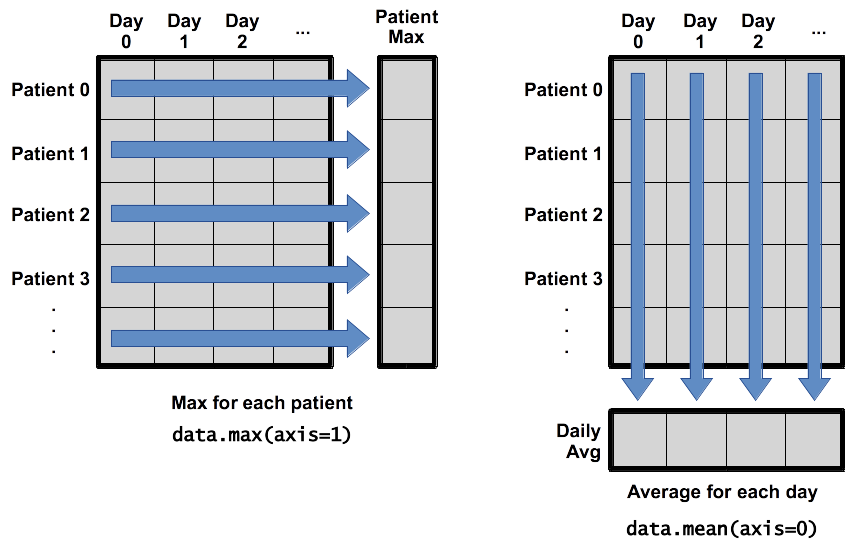
To support this functionality, most array functions allow us to specify the axis we want to work on. If we ask for the average across axis 0 (rows in our 2D example), we get:

print(np.mean(data, axis=0))

[  0.           0.45         1.11666667   1.75         2.43333333   3.15
   3.8          3.88333333   5.23333333   5.51666667   5.95         5.9
   8.35         7.73333333   8.36666667   9.5          9.58333333
  10.63333333  11.56666667  12.35        13.25        11.96666667
  11.03333333  10.16666667  10.           8.66666667   9.15         7.25
   7.33333333   6.58333333   6.06666667   5.95         5.11666667   3.6
   3.3          3.56666667   2.48333333   1.5          1.13333333
   0.56666667]

As a quick check, we can ask this array what its shape is:

print(np.mean(data, axis=0).shape)

(40,)

The expression (40,) tells us we have an N×1 vector, so this is the average inflammation per day for all patients. If we average across axis 1 (columns in our 2D example), we get:

patients_avg = np.mean(data, axis=1)
patients_avg

[ 5.45   5.425  6.1    5.9    5.55   6.225  5.975  6.65   6.625  6.525
  6.775  5.8    6.225  5.75   5.225  6.3    6.55   5.7    5.85   6.55
  5.775  5.825  6.175  6.1    5.8    6.425  6.05   6.025  6.175  6.55
  6.175  6.35   6.725  6.125  7.075  5.725  5.925  6.15   6.075  5.75
  5.975  5.725  6.3    5.9    6.75   5.925  7.225  6.15   5.95   6.275  5.7
  6.1    6.825  5.975  6.725  5.7    6.25   6.4    7.05   5.9  ]

Which is the average inflammation per patient across all days.

Change In Inflammation

This patient data is longitudinal in the sense that each row represents a series of observations relating to one individual. This means that the change in inflammation over time is a meaningful concept.

The np.diff() function takes a NumPy array and returns the differences between two successive values along a specified axis. For example, a NumPy array that looks like this:

npdiff = np.array([ 0,  2,  5,  9, 14])

Calling np.diff(npdiff) would do the following calculations and put the answers in another array.

[ 2 - 0, 5 - 2, 9 - 5, 14 - 9 ]

np.diff(npdiff)

array([2, 3, 4, 5])

Which axis would it make sense to use this function along?

Solution

Since the row axis (0) is patients, it does not make sense to get the difference between two arbitrary patients. The column axis (1) is in days, so the difference is the change in inflammation – a meaningful concept.

np.diff(data, axis=1)

If the shape of an individual data file is (60, 40) (60 rows and 40 columns), what would the shape of the array be after you run the diff() function and why?

Solution

The shape will be (60, 39) because there is one fewer difference between columns than there are columns in the data.

How would you find the largest change in inflammation for each patient? Does it matter if the change in inflammation is an increase or a decrease?

Solution

By using the np.max() function after you apply the np.diff() function, you will get the largest difference between days. We can functionally compose these together.

np.max(np.diff(data, axis=1), axis=1)

array([  7.,  12.,  11.,  10.,  11.,  13.,  10.,   8.,  10.,  10.,   7.,
         7.,  13.,   7.,  10.,  10.,   8.,  10.,   9.,  10.,  13.,   7.,
        12.,   9.,  12.,  11.,  10.,  10.,   7.,  10.,  11.,  10.,   8.,
        11.,  12.,  10.,   9.,  10.,  13.,  10.,   7.,   7.,  10.,  13.,
        12.,   8.,   8.,  10.,  10.,   9.,   8.,  13.,  10.,   7.,  10.,
         8.,  12.,  10.,   7.,  12.])

If inflammation values decrease along an axis, then the difference from one element to the next will be negative. If you are interested in the magnitude of the change and not the direction, the np.absolute() function will provide that.

Notice the difference if you get the largest absolute difference between readings.

np.max(np.absolute(np.diff(data, axis=1)), axis=1)

array([ 12.,  14.,  11.,  13.,  11.,  13.,  10.,  12.,  10.,  10.,  10.,
        12.,  13.,  10.,  11.,  10.,  12.,  13.,   9.,  10.,  13.,   9.,
        12.,   9.,  12.,  11.,  10.,  13.,   9.,  13.,  11.,  11.,   8.,
        11.,  12.,  13.,   9.,  10.,  13.,  11.,  11.,  13.,  11.,  13.,
        13.,  10.,   9.,  10.,  10.,   9.,   9.,  13.,  10.,   9.,  10.,
        11.,  13.,  10.,  10.,  12.])

Broadcasting (Optional)

This is another really powerful feature of NumPy, and covers a ‘special case’ of array multiplication.

By default, array operations are element-by-element:

np.arange(5) * np.arange(5)

array([ 0,  1,  4,  9, 16])

If we multiply arrays with non-matching shapes we get an error:

np.arange(5) * np.arange(6)

Traceback (most recent call last):
  File "<stdin>", line 1, in <module>
ValueError: operands could not be broadcast together with shapes (5,) (6,)

Or with a multi-dimensional array:

np.zeros([2,3]) * np.zeros([2,4])

Traceback (most recent call last):
  File "<stdin>", line 1, in <module>
ValueError: operands could not be broadcast together with shapes (2,3) (2,4)

Arrays must match in all dimensions in order to be compatible:

np.ones([3, 3]) * np.ones([3, 3]) # Note elementwise multiply, *not* matrix multiply.

array([[ 1.,  1.,  1.],
       [ 1.,  1.,  1.],
       [ 1.,  1.,  1.]])

Except, that if one array has any Dimension size of 1, then the data is automatically REPEATED to match the other dimension. This is known as broadcasting.

So, let’s consider a subset of our inflammation data (just so we can easily see what’s going on):

subset = data[:10, :10]
subset

array([[0., 0., 1., 3., 1., 2., 4., 7., 8., 3.],
       [0., 1., 2., 1., 2., 1., 3., 2., 2., 6.],
       [0., 1., 1., 3., 3., 2., 6., 2., 5., 9.],
       [0., 0., 2., 0., 4., 2., 2., 1., 6., 7.],
       [0., 1., 1., 3., 3., 1., 3., 5., 2., 4.],
       [0., 0., 1., 2., 2., 4., 2., 1., 6., 4.],
       [0., 0., 2., 2., 4., 2., 2., 5., 5., 8.],
       [0., 0., 1., 2., 3., 1., 2., 3., 5., 3.],
       [0., 0., 0., 3., 1., 5., 6., 5., 5., 8.],
       [0., 1., 1., 2., 1., 3., 5., 3., 5., 8.]])

Let’s assume we wanted to multiply each of the 10 individual day values in a patient row for every patient, by contents of the following array:

multiplier = np.arange(1, 11)
multiplier

array([1, 2, 3, 4, 5, 6, 7, 8, 9, 10])

So, the first day value in a patient row is multiplied by 1, the second day by 2, the third day by 3, etc.

We can just do:

subset * multiplier

array([[ 0.,  0.,  3., 12.,  5., 12., 28., 56., 72., 30.],
       [ 0.,  2.,  6.,  4., 10.,  6., 21., 16., 18., 60.],
       [ 0.,  2.,  3., 12., 15., 12., 42., 16., 45., 90.],
       [ 0.,  0.,  6.,  0., 20., 12., 14.,  8., 54., 70.],
       [ 0.,  2.,  3., 12., 15.,  6., 21., 40., 18., 40.],
       [ 0.,  0.,  3.,  8., 10., 24., 14.,  8., 54., 40.],
       [ 0.,  0.,  6.,  8., 20., 12., 14., 40., 45., 80.],
       [ 0.,  0.,  3.,  8., 15.,  6., 14., 24., 45., 30.],
       [ 0.,  0.,  0., 12.,  5., 30., 42., 40., 45., 80.],
       [ 0.,  2.,  3.,  8.,  5., 18., 35., 24., 45., 80.]])

Which gives us what we want, since each value in multiplier is applied successively to each value in a patient’s row, but over every patient’s row. So, every patient’s first value is multiplied by 1, every patient’s second value is multiplied by 2, etc.

Since multiplier has only one dimension, but the size of that dimension matches our number of days (the second dimension of subset), broadcasting automatically repeats the data in multiplier to match the number of patients (the first dimension in subset) so the * operation can be applied over arrays of equal shape.

Key Points

• Processing NumPy arrays is generally much faster than processing Python lists.

• NumPy arrays have specialised capabilities to support complex mathematical operations, and are less flexible that Python lists.

• Slicing NumPy arrays returns a reference to the original dataset, not a copy of it like with Python lists.

• NumPy arrays only hold elements of a single data type and are generally fixed in size.

• Use numpy.mean(array), numpy.max(array), and numpy.min(array) to calculate simple statistics.

• Use numpy.mean(array, axis=0) or numpy.mean(array, axis=1) to calculate statistics across the specified axis.

• Broadcasting allows you to apply an operation to two arrays of different shape, repeating the data in an array of a one-long dimension to match the larger array.